Verification

Introduction

In the context of natural phenomena modelling, verification refers to the process of confirming that the final program’s output mathematically corresponds to the analytically derived, expected outcome. Validation refers to the process of confirming that the model can, to some degree of accuracy, model the real phenomena it is meant to predict. In simplified terms, verification tests simplified cases that can be modelled both computationally and analytically, and compares the results. Validation tests real world, complex cases that can only be studied computationally and historically. These two processes give greater confidence (but not guarantee) that the model is performing as it is expected, and can reliably predict future events.

ASTM E1355 Standard Guide for Evaluating the Predictive Capability of Deterministic Fire Models (2018) defines model verification as “the process of determining that the implementation of a calculation method accurately represents the developer’s conceptual description of the calculation method and solution to the calculation method.” Slightly different definitions of model verification are used by other standards in other industries, but in general verification involves assessing whether the underlying mathematical formulation is correctly implemented in the source code - or “is the math right”. ASTM E1355 Standard Guide for Evaluating the Predictive Capability of Deterministic Fire Models (2018) defines model validation as “the process of determining the degree to which a calculation method is an accurate representation of the real-world from the perspective of the intended uses of the calculation method.”

Verification and validation of wildfire spread models has its own intricacies and particularities, as the range of methodologies that can be employed to model wildfire spread are broad and varied. Sullivan categorises the plethora of models in the literature as spanning a spectrum between empirical (purely relying on experimental correlations and interpolations) and physical (purely relying on conservation laws and heat and mass transfer laws). Most wildfire models are somewhere inbetween, with some degree of physical reasoning and calibration required by all models. ELMFIRE would be classified as a semi-empirical model, as it primarily uses physically-derived equation with empirical, experiment-driven parameterization.

Model verification is typically approached by simulating simple canonical problems and comparing model outputs to exact solutions, where available. ELMFIRE has been subjected to extensive model verification exercises since development began in 2010. In an effort to promote transparency and authenticity, ELMFIRE’s mathematical formulation is documented in the Technical Reference, its source code is maintained in a public Git repository, and several model verification test cases.

This guide will present the results of a verification and validation study of ELMFIRE. A series of simplified cases will first be presented, with quantitative and qualitative comparison of the computational and analytical results. Following that, a series of historical wildfires will be modelled in ELMFIRE. The results will be compared to establish ELMFIRE’s ability to work on real, complex landscapes.

Verification Test Cases

The verification of ELMFIRE will be based on the WUI-NITY project verification guide (WUI-NITY 2), where a wildfire spread model verification method is described, and later applied in a benchmarking study. The verification test suggests small landscapes with five simplified scenarios:

• “Point”: Uniform fuel, flat landscape, zero wind, ignition at the center of the landscape.

• “Windy”: Uniform fuel, flat landscape, northern wind, ignition at the north part of the landscape.

• “Valley”: Uniform fuel, a shallow landscape rise to the east and a steep rise to the west, zero wind, ignition at the center of the landscape.

• “Fuel Quadrant”: Different fuels at each quadrant of the landscape, flat landscape, zero wind, ignition at the center of the landscape.

• “Complex”: (an amalgamation of the previous cases) Different fuels at each quadrant of the landscape, a shallow landscape rise to the east and a steep rise to the west, northern wind, ignition at the center.

Each of these tests verifies the model against a separate parameter, with the final one superimposing the previous cases to test their interaction. For this verification guide, additional tests are proposed to expand the parameters being examined and verified. These extra tests follow from the submodel breakdown identified in the main guide.

• “Moisture Quadrant”: Uniform fuel, with different fuel moisture values at each landscape quadrant.

• “Canopy”: Same as “Windy” case, with canopy values included.

• “Firebrands”: Uniform fuel, flat landscape, northern wind, line ignition at the north, with firebrand generation included.

• “Overnight”: Same as “Point” with an overnight burn duration.

• “Suppression”: Same as “Point” with suppression to the south of the ignition.

The expected outcomes of each case are shown in Fig. 7. The original five cases are colored orange, and the four new cases are colored blue. Some of the original figures have been altered compared to the original source. Based on these cases, appropriate weather, topography and fuel files were created to run each simulation.

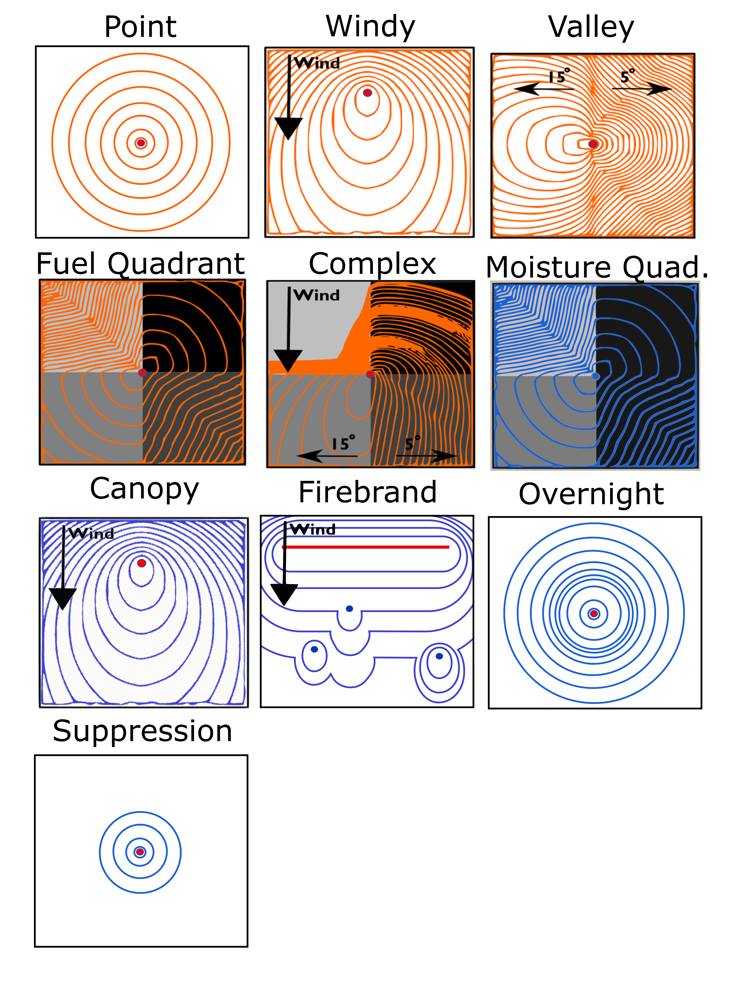
Fig. 7 The nine verification cases of this study. The orange fire fronts represent the original five cases, and the blue fire fronts represent the new cases. Adapted from WUI-NITY 2.

The details of each case are described in Table 4. All the raster inputs are 126 x 126 cells with 30m cell size. Wind magnitude and direction is spatially constant. Simulation DT is 1 minute. Wind is specified at 10m height. 10-hour and 100-hour fuel moistures are 7% and 8% for all fuels and cases, live herbaceous fuel moisture is set to 90% and live woody fuel moisture is set to 60%. Where analytical solutions for the rate of spread can be acquired, they are calculated through the Rothermel model and the BEHAVE program. All isochrones shown in the later sections are hourly.

Table 4 Simulation parameters of each verification case. Changes in fuel types between cases occur to generate faster or slower wildfires, for better visualisation or comparison.

Case	Topography	Fuel (FBFM13)	CC (%)	CBH (m×10)	CBD (kg/m³×100)	CH (m×10)	Wind (mph)	1h FMC	Firebrands	Diurnal	Suppression
Point	Flat	3	0	0	0	0	0.0	6	off	off	off
Windy	Flat	5	0	0	0	0	5	6	off	off	off
Valley	5° east, 15° west	3	0	0	0	0	0.0	6	off	off	off
Fuel Quadrant	Flat	8, 7, 4, 2	0	0	0	0	0.0	6	off	off	off
Complex	5° east, 15° west	8, 7, 4, 2	0	0	0	0	5	6	off	off	off
Moisture Quad.	Flat	3	0	0	0	0	0.0	6, 12, 18, 25	off	off	off
Canopy	Flat	5	80	16	56	55	1, 6, 12	6	off	off	off
Firebrand	Flat	3	0	0	0	0	5	6	on	off	off
Overnight	Flat	3	0	0	0	0	0.0	6	off	72 h runtime	off
Suppression	Flat	3	0	0	0	0	0.0	6	off	off	on

To maintain accuracy between versions, and ensure that subsequent changes do not affect the verification results, we have included scripts to automatically run and verify all cases below. The verification/GUIDE/run_verification.sh script runs all cases and compares them with the analytically derived results, highlighting discrepancies and similarities. The output of this script is a table summarising the critical values of each case.

Case                Metric                          Target   ELMFIRE    %err  Result
------------------------------------------------------------------------------------
Point               head ROS                         1.510     1.512     0.1  PASS
Windy               head ROS                         3.635     3.644     0.3  PASS
Windy               L/W ratio                        1.240     1.248     0.6  PASS
Valley              head ROS (5 deg, east)           1.920     1.924     0.2  PASS
Valley              head ROS (15 deg, west)          5.370     5.374     0.1  PASS
Quadrant            FB8 head ROS                     0.080     0.080    -0.6  PASS
Quadrant            FB7 head ROS                     0.472     0.471    -0.3  PASS
Quadrant            FB4 head ROS                     1.492     1.493     0.1  PASS
Quadrant            FB2 head ROS                     0.871     0.872     0.1  PASS
MoistureQuad        ROS @ 6%                         1.511     1.512     0.1  PASS
MoistureQuad        ROS @ 12%                        1.089     1.090     0.1  PASS
MoistureQuad        ROS @ 18%                        0.801     0.801     0.0  PASS
MoistureQuad        ROS @ 25%                        0.000     0.000       -  PASS
Canopy-1mph         crown class                      0.000     0.000       -  PASS
Canopy-1mph         max ROS                          1.809     1.745    -3.5  PASS
Canopy-5mph         crown class                      1.000     1.000     0.0  PASS
Canopy-5mph         max ROS                         10.060    10.084     0.2  PASS
Canopy-10mph        crown class                      2.000     2.000     0.0  PASS
Canopy-10mph        max ROS                         35.300    35.443     0.4  PASS
Complex             max ROS (qualitative)                -    12.896       -  n/a
Firebrands          firebrands (cell)             8450.000 12198.000    44.4  FAIL
Firebrands          ln-distance mu                   2.420     2.411    -0.4  PASS
Firebrands          ln-distance sigma                1.310     1.300    -0.7  PASS
Overnight           reduction starts (hr)           17.500    17.750     1.4  PASS
Overnight           reduction ends (hr)              7.500     7.750     3.3  PASS
Suppression-extendedtime at simulation end       88200.000 83988.000    -4.8  PASS
Suppression-initial fraction contained               0.540     0.569     5.4  PASS

Point

Goal.

Verify baseline isotropic spread in the absence of wind and slope.

Setup.

Flat terrain and no wind. BEHAVE (Rothermel surface model) inputs:

• Fuel Model: FB3 (3) Tall Grass (static)

• 1-h fuel moisture: 6%

• 20-ft wind speed: 0 mph

• Slope steepness: 0%

Expected outcome.

Circular isochrones with constant rate of spread.

Result.

Figure  Fig. 8 shows circular fire fronts. The estimated rate of spread is 1.51 m/min, matching BEHAVE.

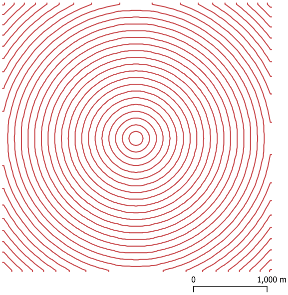
Fig. 8 ELMFIRE simulation of verification case “Point”

Windy

Goal.

Verify wind-driven elliptical spread and agreement with an analytical/BEHAVE-based isochrone.

Method.

Compute the wind adjustment factor (WAF) to convert 20-ft wind to midflame wind, then compare BEHAVE-derived spread metrics and analytical isochrones against ELMFIRE.

Wind adjustment factor.

For uncovered fuels (no or sparse canopy):

\[\begin{equation} WAF_u = \frac{1.83}{ \ln\left( \frac{20 + 0.36H}{0.13H} \right)} \end{equation}\]

Where H is the fuel depth height in feet. If canopy is present, the sheltered WAF is used. All WAF values are constrained between 0.1 and 1.

\[\begin{equation} WAF_s = \frac{0.555}{\sqrt{\frac{H(CH-CBH)}{CH}} \ln\left( \frac{20 + 0.36H}{0.13H} \right)} \end{equation}\]

Recall that the point fire spread can be characterised by an ellipse whose Length over Width ratio can be found by:

\[\begin{equation} \frac{L}{W} = \min \left[ 0.936\, e^{0.1147\, U_{mf,e}} + 0.461\, e^{-0.0692\, U_{mf,e}} - 0.397,\; 8 \right] \end{equation}\]

Setup.

Uniform topography and constant wind. BEHAVE inputs:

• Fuel Model: FB5 (5) Brush (static)

• 1-h fuel moisture: 6%

• 10-h fuel moisture: 7%

• 20ft wind speed: 6 mph

• Slope steepness: 0%

Expected (BEHAVE/analytical).

• Wind adjustment factor: 0.42

• Head rate of spread: 3.66 m/min

• Midflame windspeed: 2.5 km/h

• \(L/W\): 1.24

Result (ELMFIRE).

• Head rate of spread: 3.644 m/min

• \(L/W\): 1.248

Comparison.

The match is almost identical, supporting correct implementation of wind-driven elliptical spread.

Valley

Goal.

Verify slope-driven spread and the Huygens construction (successive isochrones consistent with point-source expansions).

Setup.

Two slopes (5% and 15%), no wind. BEHAVE inputs:

• Fuel Model: FB3 (3) Tall Grass (static)

• 1-h fuel moisture: 6%

• 20ft wind speed: 0 mph

• Slope steepness: 5% / 15%

Expected (BEHAVE).

• Head rate of spread (5%): 1.92 m/min

• \(L/W\) (5%): 1.01

• Head rate of spread (15%): 5.37 m/min

• \(L/W\) (15%): 1.07

Result (ELMFIRE).

• Head rate of spread (5%): 1.92 m/min

• Head rate of spread (15%): 5.37 m/min

Huygens check.

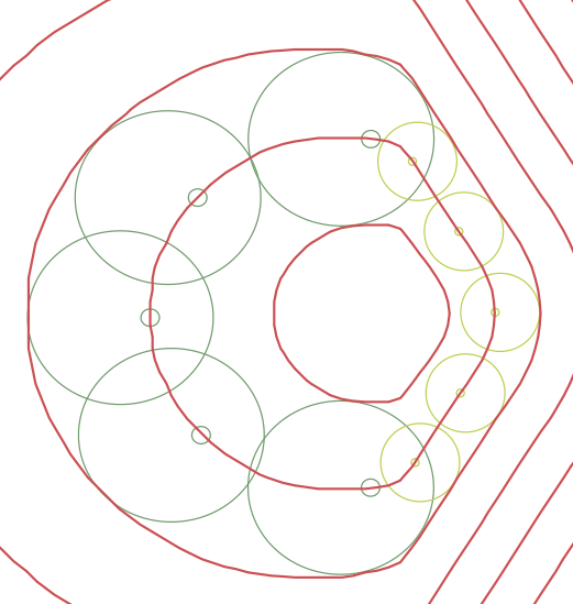
Rather than estimating \(L/W\) directly from the composite isochrones, BEHAVE-derived \(L/W\) values are used to draw 1-hour point-spread ellipses for each slope and overlay them on a given isochrone.

• Head \(L/W\) (5%): 1.01

• Head \(L/W\) (15%): 1.07

Comparison.

Overlaying the 1-hour point spreads onto an isochrone aligns well with the next ELMFIRE outline (Figure  Fig. 9).

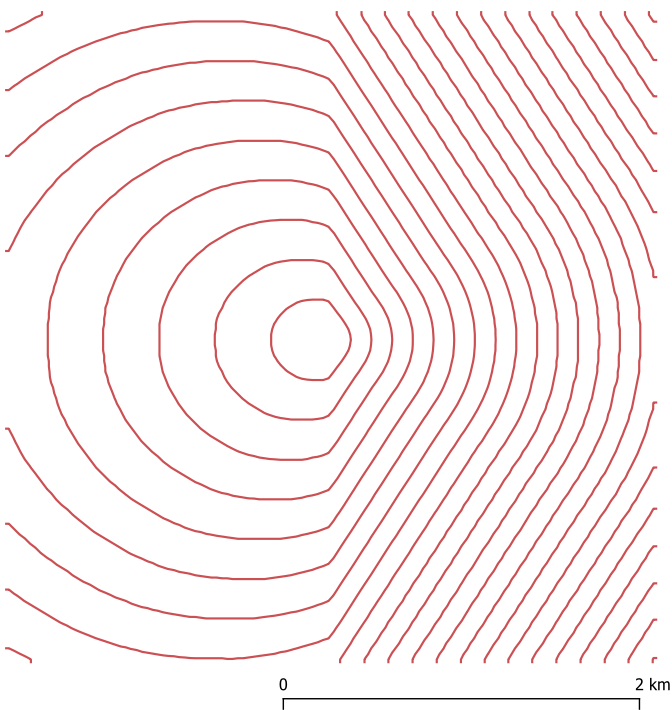
Fig. 9 Left: The “Valley” verification case in ELMFIRE. Right: the 5° and 15° incline point ignition ellipses overlapped between two isochrones, with great match.

Quadrant

Goal.

Verify that ELMFIRE handles spatially varying fuel models correctly by checking (i) that the composite fire perimeter remains physically reasonable when it crosses fuel boundaries and (ii) that the head rate of spread within each fuel matches BEHAVE.

Setup.

Four fuel models arranged in quadrants, no wind, no slope. BEHAVE inputs:

• Fuel Models:

  1. FB2 (2) Timber (grass and understory)

  2. FB4 (4) Chaparral (6 feet)

  3. FB7 (7) Southern Rough

  4. FB8 (8) Closed Timber Litter

• 1-h fuel moisture: 6%

• 10-h fuel moisture: 7%

• 100-h fuel moisture: 8%

• Live herbaceous fuel moisture: 60%

• Live woody fuel moisture: 90%

• 20ft wind speed: 0 mph

• Slope steepness: 0%

Expected (BEHAVE).

• FB2 head rate of spread: 0.871 m/min

• FB4 head rate of spread: 1.492 m/min

• FB7 head rate of spread: 0.472 m/min

• FB8 head rate of spread: 0.080 m/min

Result (ELMFIRE).

• FB2 head rate of spread: 0.872 m/min

• FB4 head rate of spread: 1.974 m/min

• FB7 head rate of spread: 0.551 m/min

• FB8 head rate of spread: 0.080 m/min

Comparison.

ELMFIRE matches BEHAVE closely for FB2 and FB8, while FB4 and FB7 exhibit higher ELMFIRE spread rates under the same inputs (discrepancy is currently being investigated). Qualitatively, the perimeter shape remains consistent across fuel boundaries (no nonphysical kinks or discontinuities), indicating that the multi-fuel coupling behaves sensibly; remaining quantitative differences are investigated further in Section  Complex.

Complex

The complex case is beyond analytical solution or comparison to an ideal solution and is the primary reason why one needs wildfire spread models. This case is added for qualitative review, to showcase the compilation of previous cases and investigate whether the results do linearly add to one another. As such, it is expected to see fast southward spread, with higher spread eastward (toward the higher slope) and towards the faster-spread fuel model. Indeed, that is exactly what ELMFIRE predicts.

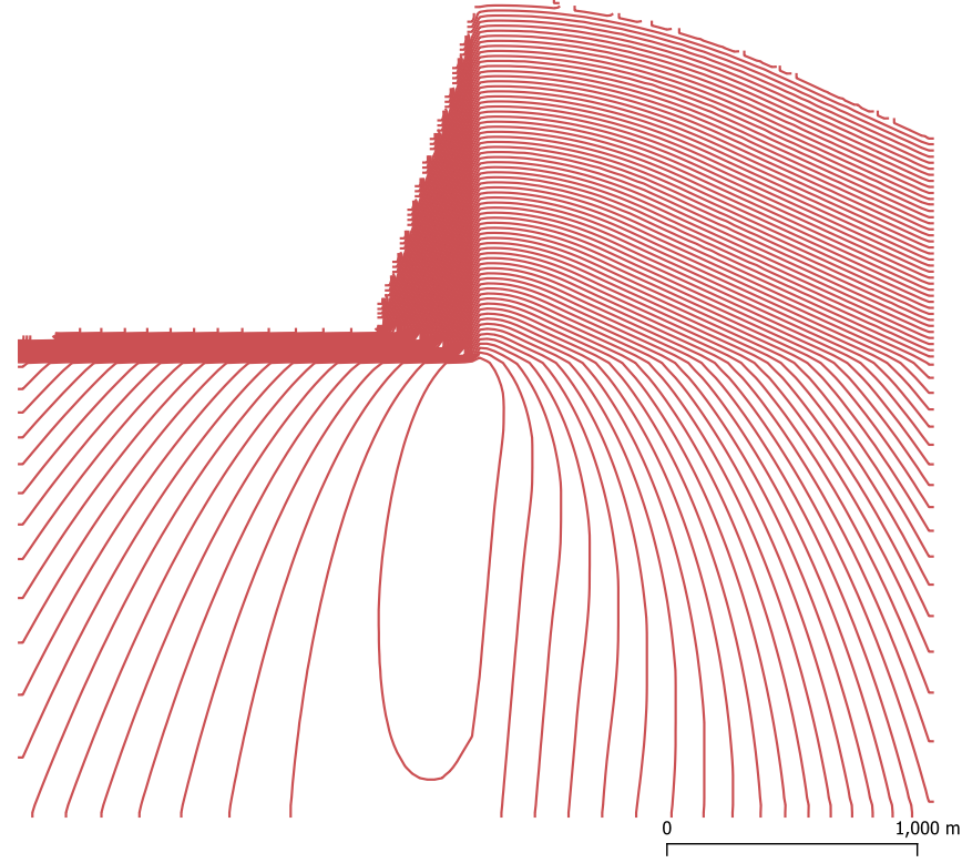
Fig. 10 The “Complex” verification case results from ELMFIRE.

Moisture Quad

Goal.

Verify that spatially varying fuel moisture inputs are parsed and applied correctly in ELMFIRE.

Setup.

Uniform fuel model (FB3) with quadrant-wise 1-h fuel moisture (6%, 12%, 18%, 25%), no wind, no slope. BEHAVE inputs:

• Fuel Model: FB3 (3) Tall grass (static)

• 1-h fuel moisture: 6%, 12%, 18%, 25%

• 20ft wind speed: 0 mph

• Slope steepness: 0%

Expected (BEHAVE).

• 6%: 1.511 m/min

• 12%: 1.089 m/min

• 18%: 0.801 m/min

• 25%: 0 m/min

Result (ELMFIRE).

• 6%: 1.511 m/min

• 12%: 1.089 m/min

• 18%: 0.801 m/min

• 25%: 0 m/min

Comparison.

ELMFIRE matches BEHAVE for all four moisture values. In particular, the 25% quadrant (approximately the moisture of extinction for fuel model 3) correctly yields zero spread, verifying correct interpretation and application of spatially varying fine fuel moisture.

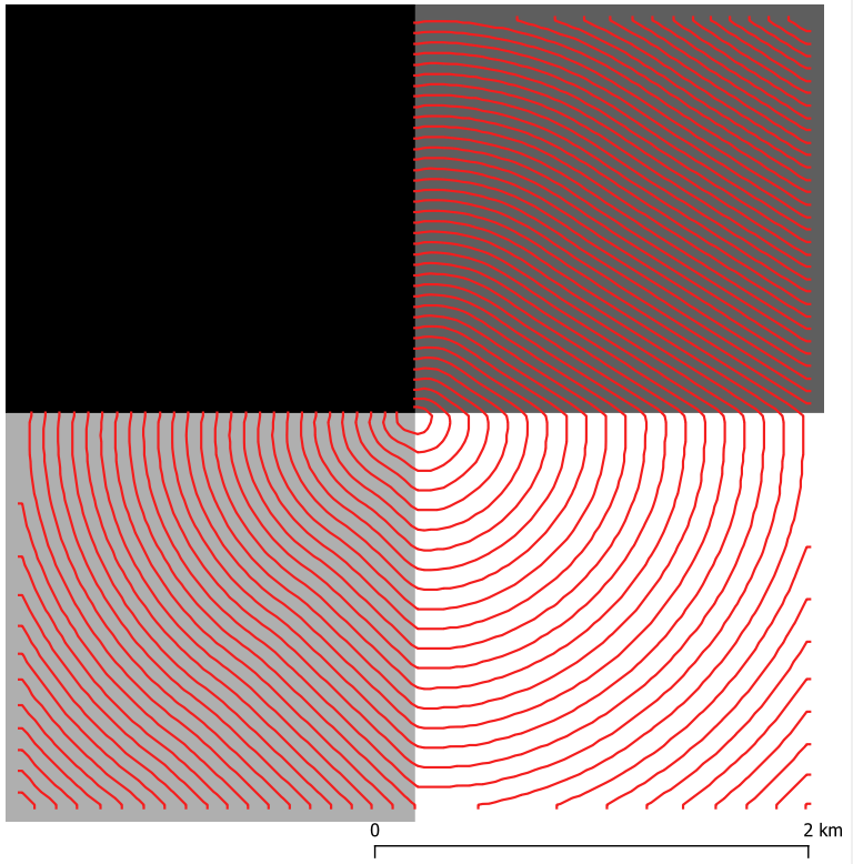
Fig. 11 The “Moisture Quadrant” verification case results in ELMFIRE. Fuel moisture is plotted on the background with values ranging from 6 (white) to 25 (black).

Canopy

Goal.

Verify crown fire initiation/classification (surface vs. passive vs. active crown fire) and crown spread rate calculations in ELMFIRE under nonzero canopy conditions.

Setup.

A uniform domain with canopy parameters enabled. BEHAVE is used to obtain surface fire spread rate and fireline intensity, then the crown fire equations in Section  Canopy Fires are applied analytically for comparison. Inputs:

• Fuel Model: FB3 (3) Tall Grass (static)

• 1-h fuel moisture: 6%

• 20ft wind speed: 1, 5, 10 mph

• Slope steepness: 0%

• Foliar Moisture Content: 90%

• Canopy Base Height: 1.6 m

• Canopy Height: 5.5 m

• Canopy Bulk Density: 0.10 \(kg\,m^{-3}\)

• Canopy Cover: 80%

Expected (analytical, using BEHAVE surface fire outputs).

1 mph.

• Head rate of spread (surface): 1.809 m/min

• Critical crown rate of spread \(R_0\): 30.0 m/min

• Predicted active crown rate of spread \(R_C\):4.44 m/min

• Criteria for active crowning \(CAC\): 0.15

• Critical Fireline Intensity \(I_0\): 477.3 kW/m

• Predicted Fireline Intensity \(I\): 254.4 kW/m

• Crown Fire: None

• Predicted final rate of spread \(R\): 1.809 m/min

5 mph.

• Head rate of spread (surface): 3.44 m/min

• Critical crown rate of spread \(R_0\): 30.0 m/min

• Predicted active crown rate of spread \(R_C\): 18.9 m/min

• Criteria for active crowning \(CAC\): 0.63

• Critical Fireline Intensity \(I_0\): 477.3 kW/m

• Predicted Fireline Intensity \(I\): 449.0 kW/m

• Crown Fire: Passive

• Predicted final rate of spread \(R\): 10.06 m/min

10 mph.

• Head rate of spread (surface): 5.26 m/min

• Critical crown rate of spread \(R_0\): 30.0 m/min

• Predicted active crown rate of spread \(R_C\): 35.3 m/min

• Criteria for active crowning \(CAC\): 1.18

• Critical Fireline Intensity \(I_0\): 477.3 kW/m

• Predicted Fireline Intensity \(I\): 685.8 kW/m

• Crown Fire: Active

• Predicted final rate of spread \(R\): 35.3 m/min

Result (ELMFIRE).

1 mph.

• Head rate of spread: 1.745 m/min

• Crown Fire: None

5 mph.

• Head rate of spread: 10.08 m/min

• Crown Fire: Passive

10 mph.

• Head rate of spread: 35.4 m/min

• Crown Fire: Active

Comparison.

The 5 mph case transitions to passive crown fire with a spread rate consistent with the analytical crown prediction. The 1 mph case remains a surface fire with ELMFIRE head rate of spread and fireline intensity in close agreement with the surface-fire expectation. The 10 mph case produces active crown fire at the head fire.

As such, ELMFIRE can be considered verified for crown fire spread classification and calculation.

Firebrand

Goal.

Verify that ELMFIRE correctly (i) samples user-defined lognormal firebrand transport distances and (ii) computes Eulerian ember flux magnitudes consistent with the analytical formulation.

Setup.

Firebrand generation, transport, and ignition (“spotting”) are supported in multiple modes in ELMFIRE. In this case, the most physical options are chosen, limiting the required user inputs. This means that spotting is setup as:

    &SPOTTING
ENABLE_SPOTTING                      = .TRUE.
USE_SUPERSEDED_SPOTTING              = .FALSE.
GENERATION_MODEL                     = 'PER-MW'
SPOTTING_DISTANCE_MODEL              = 'EMPIRICAL'
ACCUMULATION_MODEL                   = 'LAGRANGIAN'
IGNITION_MODEL                       = 'DIRECT'
ENABLE_SURFACE_FIRE_SPOTTING         = .TRUE.
SURFACE_FIRE_SPOTTING_PERCENT(:)     = 100
CRITICAL_SPOTTING_FIRELINE_INTENSITY = 200.0
PIGN                                 = 1.0
/

Expected (analytical).

(1) Lagrangian lognormal transport sampling. For a run using the predefined empirical (Sardoy) lognormal distribution, the distance sampling procedure described in Section  Transport is applied. A simulation that includes firebrands produces spotting_stats_0000001.csv, logging each firebrand trajectory and, critically here, its calculated travel distance.

A centerline cell in a symmetric domain is used so the verification analogue is effectively 1D.

The (representative) per-cell inputs are:

• 20-ft wind speed (\(U_{20}\)): 5 mph

• Fireline intensity (\(I_b\)): 2035 kW/m

• Fuel Model: 3

• Cell size (\(C\)): 30 m

• Rate of Spread: 14.4 m/min

The total ember emitting time from this cell is the maximum between the total residence time as per the Rothermel model, and the total time taken for the fire to cross the cell. For fuel model 3:

\[\Delta t_R = 15.3 s\]

\[\Delta T_{ROS}=\frac{30\times60}{14.4}=125s\]

The expected total ember count emitted from the cell per step is:

\[N=33.3\times I_{b,MW}\times \Delta t=8450\]

To compute the predicted travel distance, we refer to Section Transport. The Froude number is computed by:

\[Fr = \frac{U_{20}}{\sqrt{gL_c}}\;\;\;\;\;L_c=\frac{I_b}{\rho_\infty C_{pg} \tau_\infty \sqrt{g}}\]

(using constants \(g=9.81\), \(\rho_\infty = 1.1\), \(C_{pg} = 1\), and \(\tau_\infty = 300\)), giving \(L_c = 1.56\,\mathrm{m}\) and \(Fr = 0.56\).

Downwind and spanwise distribution parameters then are:

\[\mu_d=1.47\frac{(0.001I_b)^{0.54}}{U_{10}^{0.55}}+1.14\]

\[\sigma_d=0.86\frac{U_{10}^{0.44}}{(0.001I_b)^{0.21}}+0.19\]

\[\mu_s=0\]

\[\sigma_s=0.92L_c\]

As such, we expect a transport distance distribution that follows a lognormal distribution with:

\[\mu_d=2.42\]

\[\sigma_d=1.31\]

Comparison.

The logged Lagrangian lognormal transport distances match the independently calculated values exactly, validating the lognormal sampling implementation. For the Eulerian mode, the predicted and simulated ember flux values are of similar magnitude and follow the expected downwind decay; differences are largest for the highest-flux cell and are attributable to using averaged/representative \(I_b\) in the analytical calculation and to per-cell variability in the simulated fireline intensity. Overall, the transport component of the Eulerian spotting model and its associated submodules are considered verified.

Notes on ignition.

For the Lagrangian model, ignition is a direct per-firebrand probability and does not require verification. For the Eulerian model, the ignition probability depends on coverage density (physical model) or a user-specified probability (simple model). A dedicated verification method for the Eulerian ignition criterion is not included at this time.

Overnight

Goal.

Verify that ELMFIRE correctly computes sunrise/sunset timing and applies the diurnal (overnight) rate-of-spread reduction during the intended hours.

Setup.

The verification cases are set at the equator and span multiple simulated hours; the “Point” case in particular is configured to run for 2 simulated days. ELMFIRE does not adjust 1-h fine fuel moisture dynamically once it is read as input. To retain the effect of night-time slowing down, a constant factor of 0.1 is used to scale down the predicted rate of spread during the hours between sunset and sunrise. These hours are calculated in ELMFIRE through the NOAA Solar Position Calculations (too extensive to repeat here).

For our test case, located at the equator, the sunrise and sunset times should be at 06:00 and 18:00, regardless of the time of year. Converted to UTC, since this raster is at longitude 22.5E, yields UTC times of 04:30 and 16:30 respectively The simulation is made to start at 10:00. With a burn period length of 10 hours and a center fraction of 0.667, the expected hours that the overnight adjustment factor applies are between 17:30 and 07:30.

Result (ELMFIRE).

The resulting isochrones show the expected night-time slowdown and daytime speed-up (Figure  Fig. 12).

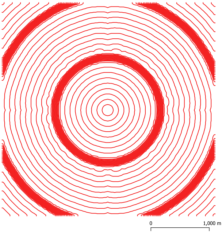
Fig. 12 The results of the “Overnight” verification case.

Comparison.

To confirm the timing, each isochrone is counted and annotated (Figure  Fig. 13). The observed transition hours closely match the expected slowdown and speed-up times, verifying that ELMFIRE correctly calculates the sunrise and sunset hours and applies the diurnal correction factor.

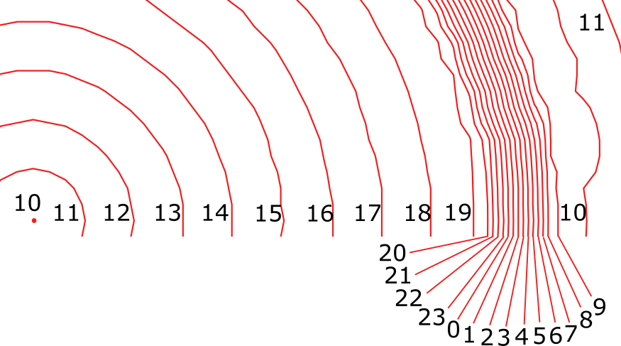
Fig. 13 An isochrone count of the Overnight verification case, with hours of arrival labelled on.

Suppression

Goal.

Verify the probabilistic initial attack containment logic and the containment evolution of both extended attack formulations.

Setup.

The “Point” case is reused as a simple geometry where spread and containment can be analyzed directly.

Initial attack (stochastic).

Expected. The initial attack submodel prescribes a probability of successful containment at the first attack opportunity. For this case, the initial attack time is set to 4800 seconds. Using a head rate of spread of 1.51 m/min, the (continuous) fire area at 4800 s is \(45800\,\mathrm{m}^2\) (11.3 acres). Because ELMFIRE uses a rasterized fire area, the area used internally is computed from the time-of-arrival raster: 69 burned cells at 30 m resolution, giving \(62100\,\mathrm{m}^2\) (15.3 acres, 6.2 hectares). The fireline intensity is 212.5 kW/m. With these values, the expected probability of containment is 54%.

Result. The verification case was run for 20000 realizations with different random seeds. About 52% of the simulated fires are contained at the initial attack time.

Comparison. The observed containment frequency (52%) is close to the expected probability (54%), verifying correct implementation of the initial attack success logic.

Extended attack – Area-Growth-Based Containment Model (deterministic).

Expected. The “Point” case is rerun with ENABLE_EXTENDED_ATTACK = .TRUE. using the Area-Growth-Based Containment Model and default parameters, except for DT_EXTENDED_ATTACK = 300. The fuel model is changed to Fuel Model 8, yielding a head ROS of approximately 0.08 m/min. For this simple geometry and uniform suppression difficulty, the expected containment progression can be evaluated independently. Full containment is expected at approximately \(88200\,\mathrm{s}\).

Result. The simulation stops at 83988 seconds with final containment of 1.0. The end time is taken from the fire stats output.

Comparison. The simulated containment time is close to the independent expectation, verifying the containment evolution of the Area-Growth-Based Containment Model for this simple geometry.

Extended attack – Spatially Explicit Suppression Model (deterministic).

Expected. The “Point” case is also used to verify the Spatially Explicit Suppression Model. The test uses a point ignition, no wind, flat terrain, uniform Fuel Model 8, and a head ROS of approximately 0.08 m/min. Full suppression capacity becomes available at 100000 seconds, with an available suppression capacity of 700 m/hr and an extended attack update interval of 3600 seconds. Indirect attack is disabled so that the test isolates the direct attack component. For this idealized case, full suppression is expected during the third direct-attack operation, at approximately \(110800\,\mathrm{s}\).

Result. ELMFIRE reaches full suppression at 100800 seconds, during the third direct-attack operation.

Comparison. The fire is fully suppressed during the third direct-attack operation at 100800 seconds, consistent with the expected behavior for this idealized case. The result verifies that the Spatially Explicit Suppression Model progressively allocates the available suppression capacity to eligible fireline segments until the active fireline is fully suppressed.

FBP Test Cases

The 2009 update to the FBP system [32] contained a set of 20 verification cases, to specifically test implementations of FBP in new models or fire spread codes. Each test varies the fuel model, wind and slope vectors, fine fuel moisture contents, and other parameters to test the correct implementation of each part of the system. The 2009* update also provides final and intermediate scalar values of the fire parameters (spread rate, fireline intensity, and fuel consumption of the surface and canopy respectively). These provided tests, and the accompanying tables of results, were instrumental in the implementation and testing of the FBP module of ELMFIRE, and the developers want to thank the authors for their foresight and for providing these cases.

As only the head fire model has been implemented in ELMFIRE, the results ignore the flank and backfire part of the FBP model, as it was not implemented. The 20 cases have been implemented in ELMFIRE and can be ran automatically, with a final verdict on the similarity of the results. At present, the maximum head rate of spread and fireline intensity are tested. a 10% error window has been introduced to allow for the effect of rounding errors (e.g. between the listed slope rise given in percent and the slope input ELMFIRE accepts in nearest integer degree).

The results are given in the table below. All tests can be found in the verification folder of ELMFIRE. To run these tests, navigate to \elmfire\verification\FBP_tests\ and run ./runme.sh. The script will clear existing results, produce the ELMFIRE input files and case folders, run ELMFIRE for each case, and compare the results with the ones in the 2009 Update. A 10% margin of error is included to account for differences in slope definition and other accuracy differences between ELMFIRE integer inputs and the float inputs. As standard, the level set mode results will be displayed, but the fire potential mode results can also be compared by running python compare.py --mode 2 (some python packages might need to be installed through pip / conda).

Table 5 Comparison of target and maximum ROS and FI values across FBP verification runs. Note that cases 13, 14, and 15 are all grass model fires, with the test cases prescribing a different grass fuel load than that hardcoded in the FBP model (\(3 kg/m^2\)). Repeating the calculations with the modified surface fuel load yields the expected FI values.

Run	\(ROS_{target}\)	\(ROS_{sim}\)	\(ROS_{error}\%\)	\(FI_{target}\)	\(FI_{sim}\)	\(FI_{error}\)%	\(ROS_{match}\)	\(FI_{match}\)
01	5.6	5.3	-4.6	3147.8	3007.8	-4.4	True	True
02	121.1	125.1	3.3	164491.3	172015.0	4.6	True	True
03	80.5	79.7	-1.0	42314.9	42367.6	0.1	True	True
04	16.7	17.6	5.4	18512.3	19853.1	7.2	True	True
05	0.0	0.0	-0.9	17.9	17.9	0.2	True	True
06	42.8	41.4	-3.2	36704.9	35544.4	-3.2	True	True
07	2.4	2.4	3.3	1490.6	1557.8	4.5	True	True
08	31.2	31.0	-0.6	11792.2	11870.6	0.7	True	True
09	13.3	13.0	-2.1	6817.1	6754.8	-0.9	True	True
10	18.1	18.0	-0.6	9474.8	9537.1	0.7	True	True
11	9.4	9.6	2.2	4010.2	4227.7	5.4	True	True
12	36.1	36.6	1.4	35166.5	36135.2	2.8	True	True
13	134.7	140.8	4.5	40408.0	14972.1	-62.9	True	False
14	0.4	0.4	8.1	24.1	46.2	91.4	True	False
15	13.3	13.4	0.5	3989.6	1420.5	-64.4	True	False
16	45.1	43.2	-4.2	105514.8	102373.2	-3.0	True	True
17	1.0	1.0	1.4	3478.6	3571.0	2.7	True	True
18	1.4	1.4	-1.4	4301.9	4318.7	0.4	True	True
19	4.4	4.3	-3.1	2687.6	2642.2	-1.7	True	True
20	17.6	17.0	-3.4	20766.5	20063.6	-3.4	True	True