Tutorial 02: fire spread in flat terrain under transient wind

This tutorial builds on Tutorial 01 which showed how to set up and run a simple model of fire spread in flat terrain under a spatially uniform and temporally constant (North) wind field. In Tutorial 02, we introduce a time-dependent, but still spatially uniform, wind field.

As with Tutorial 01, to run Tutorial 02, do the following:

cd $ELMFIRE_BASE_DIR/tutorials/02-transient_wind
./01-run.sh

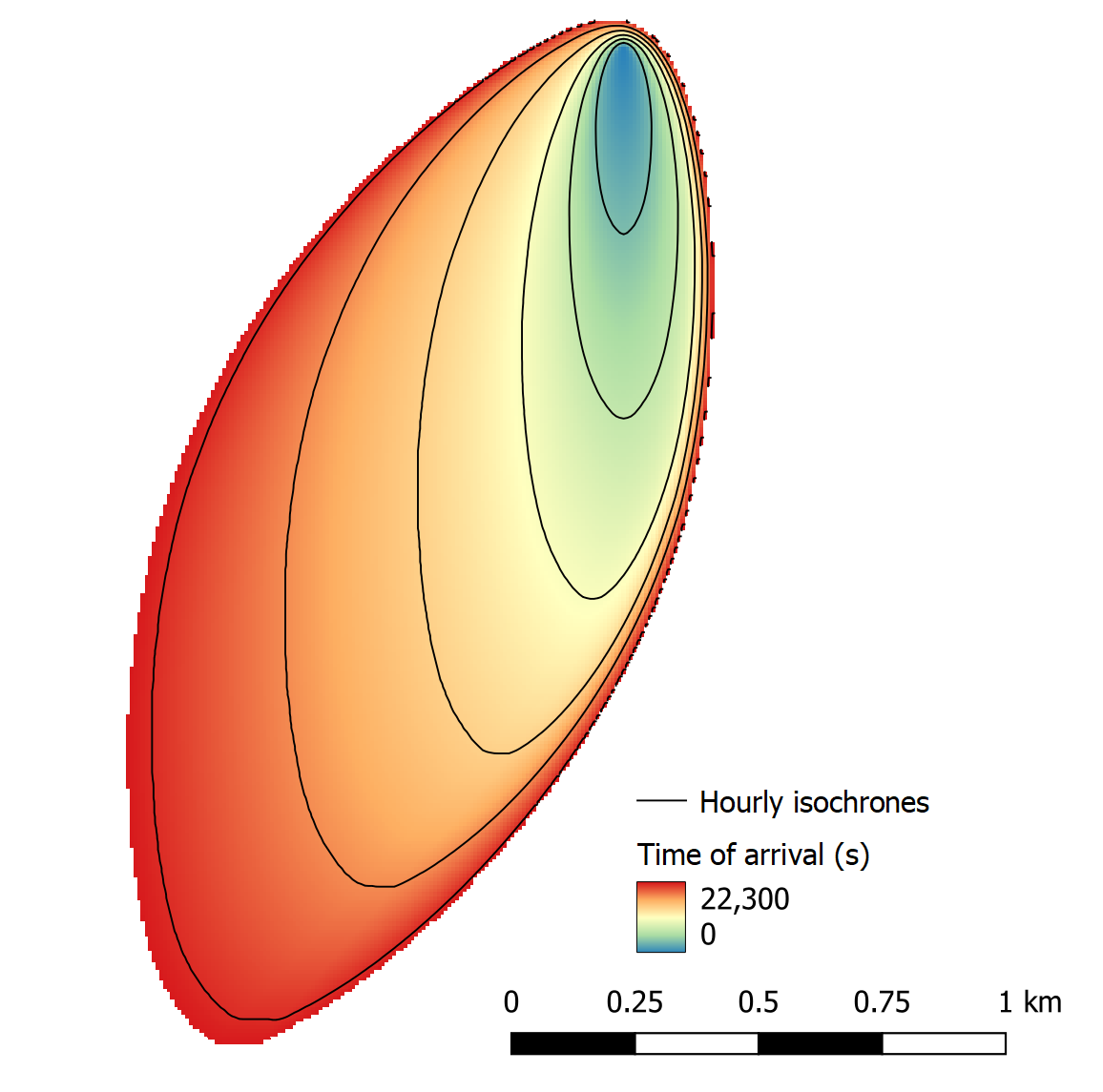
This will run a nominally 6-hr simulation with wind out of the north for the first 2 hours, shifting to the northeast between hour 2 and 4, and remaining out of the northeast for hours 4-6. The outputs, when visualized with a GIS package, should look similar to the image below which shows hourly isochrones overlaid on the time of arrival raster. Note that the fire first spreads due south for 2 hours before shifting to spread to the southwest, consistent with a wind out of the northeast:

What changes to Tutorial 01’s input deck were required to model a transient wind field? ELMFIRE reads weather and fuel moisture inputs from rasters (usually GeoTiffs). In Tutorial 01, since the weather and fuel inputs were static, the input raters had a single band that applied for the duration of the simulation. In all but idealized test cases, weather and fuel moisture inputs will change in time so multiband (sometimes called “stacked”) rasters are used to specify temporal variations. In Tutorial 02, the 01-run.sh script parses the wx.csv file and generates multiband GeoTiff rasters that are subsequently read in by ELMFIRE. Note that ELMFIRE does not directly read the wx.csv file but rather the rasters that are created by the 01-run.sh script according to the inputs specified in wx.csv, shown below:

ws,wd,m1,m10,m100,lh,lw
15,0,3,4,5,30,60
15,0,3,4,5,30,60
15,0,3,4,5,30,60
15,22.5,3,4,5,30,60
15,45,3,4,5,30,60
15,45,3,4,5,30,60
15,45,3,4,5,30,60

The header specifies that the column order is wind speed (ws), wind direction (wd), 1-hr dead fuel moisture (m1), 10-hr dead fuel moisture (m10), 100-hr dead fuel moisture (m100), live herbaceous fuel moisture (lh), and live woody fuel moisture (lw). Each row provides time-dependent values of each quantity. Here, the only quantity that varies in time is wind direction.

Since wx.csv contains no time column, how is time handled? When ELMFIRE reads in multiband rasters for temporally varying quantities, the timestep (\({\Delta}\) t ) between each band is constant and specified by the DT_METEOROLOGY keyword on the &INPUTS namelist group. Inspection of the inputs/elmfire.data file shows that DT_METEOROLOGY = 3600., meaning that the time difference between bands is 3600 s or 1 hour. This is a typical meteorology timestep when working with gridded forecast data or historical reanalysis data.

Since multiband input rasters may contain more bands that are necessary for the simulation, the number of weather bands to use in the simulation is specified in the &MONTE_CARLO namelist group via the NUM_METEOROLOGY_BANDS. The inputs/elmfire.data file contains the following namelist group to specify that 8 bands from the weather / fuel moisture rasters will be used:

&MONTE_CARLO
NUM_METEOROLOGY_TIMES = 8
/

GDAL command line utilities can be used to quickly inspect the input rasters. After navigating to the inputs directory (cd $ELMFIRE_BASE_DIR/tutorials/02-transient_wind/inputs the wind direction raster can be queried as follows:

$ gdallocationinfo -valonly wd.tif 1 1
0
0
0
22.5
45
45
45
45

This returns the expected result, namely that the wind direction raster contains 8 bands, with values in each band corresponding to the wd column specified in wx.csv. The first row of data corresponds to a simulation time of 0 s, the second row to DT_METEOROLOGY s, the third row to 2 \(\times\) DT_METEOROLOGY s, and so on. At run time, ELMFIRE uses linear interpolation to determine the value of time-dependent quantities at intermediate time steps since the numerical time step used during the fire spread simulation is typically much smaller than the timestep of the meteorological inputs.

Now is a good time to experiment with specifying various temporal variations in weather and fuel moisture fields and assessing the impact that these have on modeled fire behavior. This can be done by directly editing wx.csv and 01-run.sh. You may also want to change the ignition location, or specify multiple ignitions. This can be done by revising the &SIMULATOR namelist group in elmfire.data.in:

&SIMULATOR
NUM_IGNITIONS = 1
X_IGN(1)      = 0.0
Y_IGN(1)      = 3000.0
T_IGN(1)      = 0.0
/

Here, X_IGN and Y_IGN specify the x and y coordinates of the ignition, and T_IGN specifies the time of ignition. The index (1) specifies the ignition number. Multiple ignitions can be modeled by doing something similar to this:

&SIMULATOR
NUM_IGNITIONS = 2
X_IGN(1)      = X1
Y_IGN(1)      = Y1
T_IGN(1)      = T1
X_IGN(2)      = X2
Y_IGN(2)      = Y2
T_IGN(2)      = T2
/

where X1, Y1, T1 and X2, Y2, T2 specify the desired ignition locations and time of ignition.