Tutorial 01: fire spread in flat terrain under constant wind
One of the simplest wildland fire spread simulations, and the starting point for these tutorials, is a point ignition spreading in flat terrain under a spatially uniform and temporally invariant wind field. To run this simple model configuration, do the following:
cd $ELMFIRE_BASE_DIR/tutorials/01-constant-wind
./01-run.sh
Several output messages will scroll across the screen for a few seconds,
and when the scrolling stops the run is complete. What just happened?
Well, in short the BASH script 01-run.sh created the geospatial
inputs needed by ELMFIRE, ran ELMFIRE, and conducted basic
post-processing on ELMFIRE’s outputs. Let’s examine this more closely by
diving into the 01-run.sh BASH script (i.e., pico 01-run.sh).
The main inputs are specified between the commented lines # Begin
specifying inputs and # End inputs specification. The first three
lines
CELLSIZE=30.0 # Grid size in meters
DOMAINSIZE=12000.0 # Height and width of domain in meters
SIMULATION_TSTOP=22200.0 # Simulation stop time (seconds)
are used to specify, respectively
Cell (grid) size (m)
Computational domain size (m)
Simulation end time (s)
This will create a computational domain that is 12000.0 m / 30 m / pixel = 400 pixels by 400 lines. The simulation will terminate after 22,200 seconds (6 hours 10 minutes).
ELMFIRE takes as input both 32 bit floating point (Float32) and 16 bit
signed integer (Int16) rasters depending on the quantity being read in.
For that reason, the 01-run.sh script organizes inputs by data type,
first Float32 and then Int16. The next group of lines specifies the
values of seven Float32 inputs:
NUM_FLOAT_RASTERS=7
FLOAT_RASTER[1]=ws   ; FLOAT_VAL[1]=15.0 # 20-ft wind speed, mph
FLOAT_RASTER[2]=wd   ; FLOAT_VAL[2]=0.0  # 20-ft Wind direction, deg
FLOAT_RASTER[3]=m1   ; FLOAT_VAL[3]=3.0  # 1-hr   dead moisture content, %
FLOAT_RASTER[4]=m10  ; FLOAT_VAL[4]=4.0  # 10-hr  dead moisture content, %
FLOAT_RASTER[5]=m100 ; FLOAT_VAL[5]=5.0  # 100-hr dead moisture content, %
FLOAT_RASTER[6]=adj  ; FLOAT_VAL[6]=1.0  # Spread rate adjustment factor (-)
FLOAT_RASTER[7]=phi  ; FLOAT_VAL[7]=1.0  # Initial value of phi field
The meaning of the first five inputs is self-explanatory; the final two
inputs are adj - spread rate adjustment factor, and phi - the
initial value of the level set function \({\phi}\). Both of these
should be left at 1.0.
The value of an input parameter can be modified by changing its
corresponding FLOAT_VAL. For example, setting FLOAT_VAL[1]=10.0
would change 20-ft wind speed from 15 mph to 10 mph.
The next group of lines specifies Int16 inputs:
NUM_INT_RASTERS=8
INT_RASTER[1]=slp     ; INT_VAL[1]=0   # Topographical slope (deg)
INT_RASTER[2]=asp     ; INT_VAL[2]=0   # Topographical aspect (deg)
INT_RASTER[3]=dem     ; INT_VAL[3]=0   # Elevation (m)
INT_RASTER[4]=fbfm40  ; INT_VAL[4]=102 # Fire behavior fuel model code (-)
INT_RASTER[5]=cc      ; INT_VAL[5]=0   # Canopy cover (percent)
INT_RASTER[6]=ch      ; INT_VAL[6]=0   # Canopy height (10*meters)
INT_RASTER[7]=cbh     ; INT_VAL[7]=0   # Canopy base height (10*meters)
INT_RASTER[8]=cbd     ; INT_VAL[8]=0   # Canopy bulk density (100*kg/m3)
This group of inputs specifies values of the topography and fuel inputs needed by ELMFIRE. For consistency with units in GIS data obtained from LANDFIRE, input values of canopy height and canopy base height have units of 10 \(\times\) m, and input values of canopy bulk density have units of 100 \(\times\) kg/m3 .
The final three input lines
LH_MOISTURE_CONTENT=30.0 # Live herbaceous moisture content, percent
LW_MOISTURE_CONTENT=60.0 # Live woody moisture content, percent
A_SRS="EPSG: 32610" # Spatial reference system - UTM Zone 10
specify live herbaceous moisture content (in percent), live woody moisture content (also in percent), and the spatial reference system. For idealized cases such as the current tutorial, the latter isn’t strictly necessary but is included here for consistency with later tutorials that use real-world geospatial inputs. data.
The lines in the 01-run.sh script after # End inputs
specification generally won’t require modification. The first section
after the inputs specification script uses GDAL command line tools to burn the user-specified
input values into rasters with the CELLSIZE, DOMAINSIZE, and
A_SRS specified previously. These newly-created rasters will land in
the ./inputs directory that is created by the 01-run.sh script.
Note that the center point for these rasters is at coordinates
(0,0) and the corresponding lower left corner of the computational
domain is (-DOMAINSIZE/2, -DOMAINSIZE/2).
Next, the file elmfire.data.in is copied to
./inputs/elmfire.data, and values of various input parameters (e.g.,
A_SRS) are set accordingly. Then, ELMFIRE is run and outputs are
created in the ./outputs directory. These outputs include:
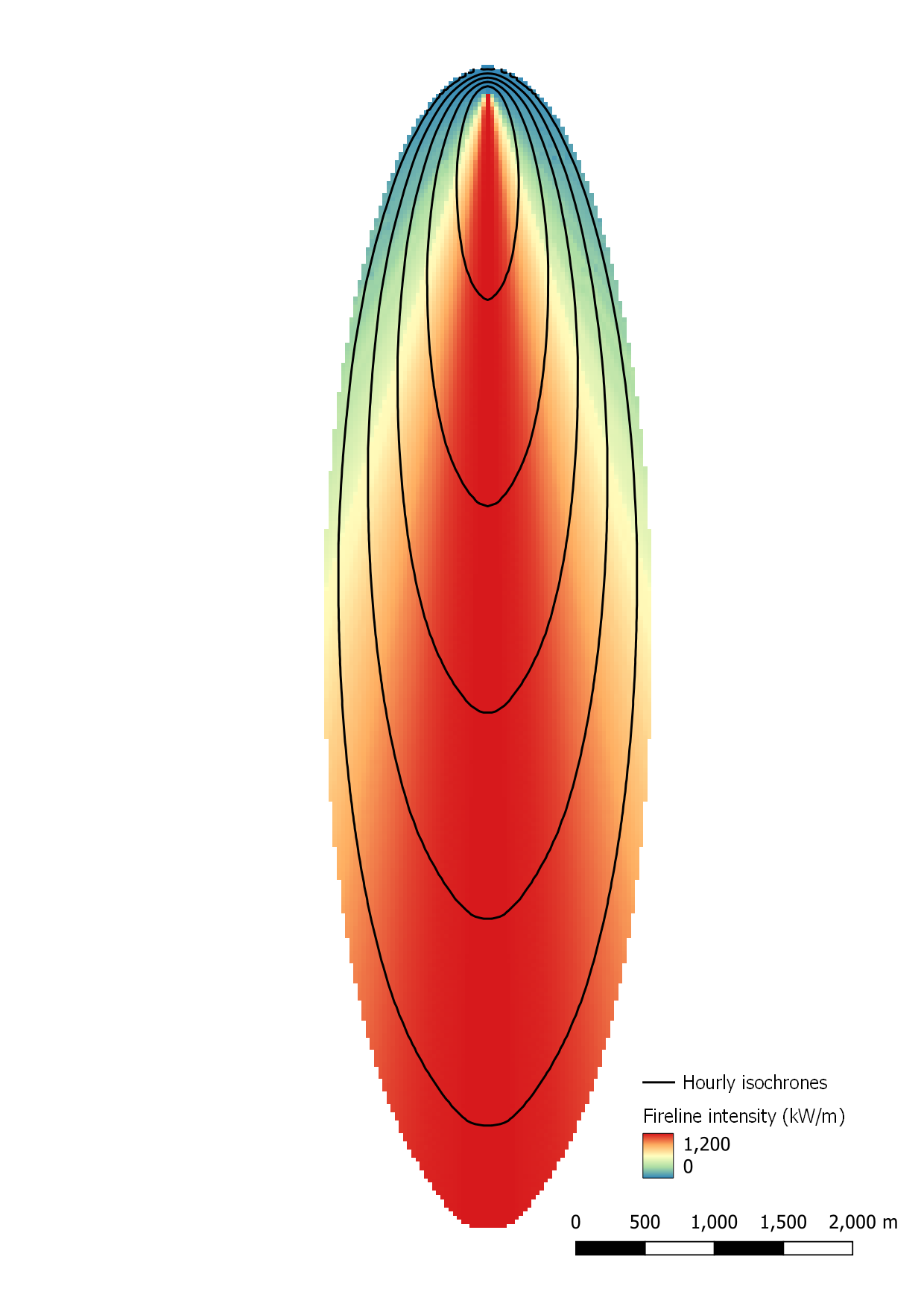
Time of arrival (s):
time_of_arrival_XXXXXXX_YYYYYYY.tifSpread rate (ft/min):
vs_XXXXXXX_YYYYYYY.tifFireline intensity (kW/m):
flin_XXXXXXX_YYYYYYY.tifHourly isochrones:
hourly_isochrones.shp
In the above naming convention:
XXXXXXXis the ensemble member number. In this tutorial there is a single ensemble member soXXXXXXX= 0000001, but ELMFIRE can be run in ensemble mode with thousands of ensemble members. In such cases, this ID is necessary to provide separate outputs for each ensemble member.YYYYYYYis the simulation time (s) at which the outputs were written out. In this tutorial, the simulation is set up to write outputs only at completion, i.e. when the simulation time exceeds the user-specifiedSIMULATION_TSTOP. Therefore, the value ofYYYYYYYwill be 22,200 seconds or greater. In some instances it is desirable to write outputs at a particular time interval, e.g. hourly, in which case and multiple outputs corresponding to different simulation times would be created for each ensemble member.
These outputs can be visualized with standard GIS software. We are particularly fond of Quantum GIS (QGIS), and will be using QGIS throughout for visualization purposes. The figure below shows a sample visualization of ELMFIRE outputs from this tutorial - fireline intensity with a spectral color ramp and hourly isochrones in front:
If you have been able to follow this tutorial and generate a simple map similar to that above, then congratulations, you are on your way to doing some really cool wildland fire modeling stuff!