Monte Carlo Analysis
Keywords controlling Monte Carlo parameters are specified in the
&MONTE_CARLO namelist group. Several types of Monte Carlo
simulations can be performed with ELMFIRE. Point source ignitions may be
placed randomly across the landscape, wind and weather inputs may be
varied stochastically, and input rasters may be spatially and temporally
perturbed.
Randomized ignition locations
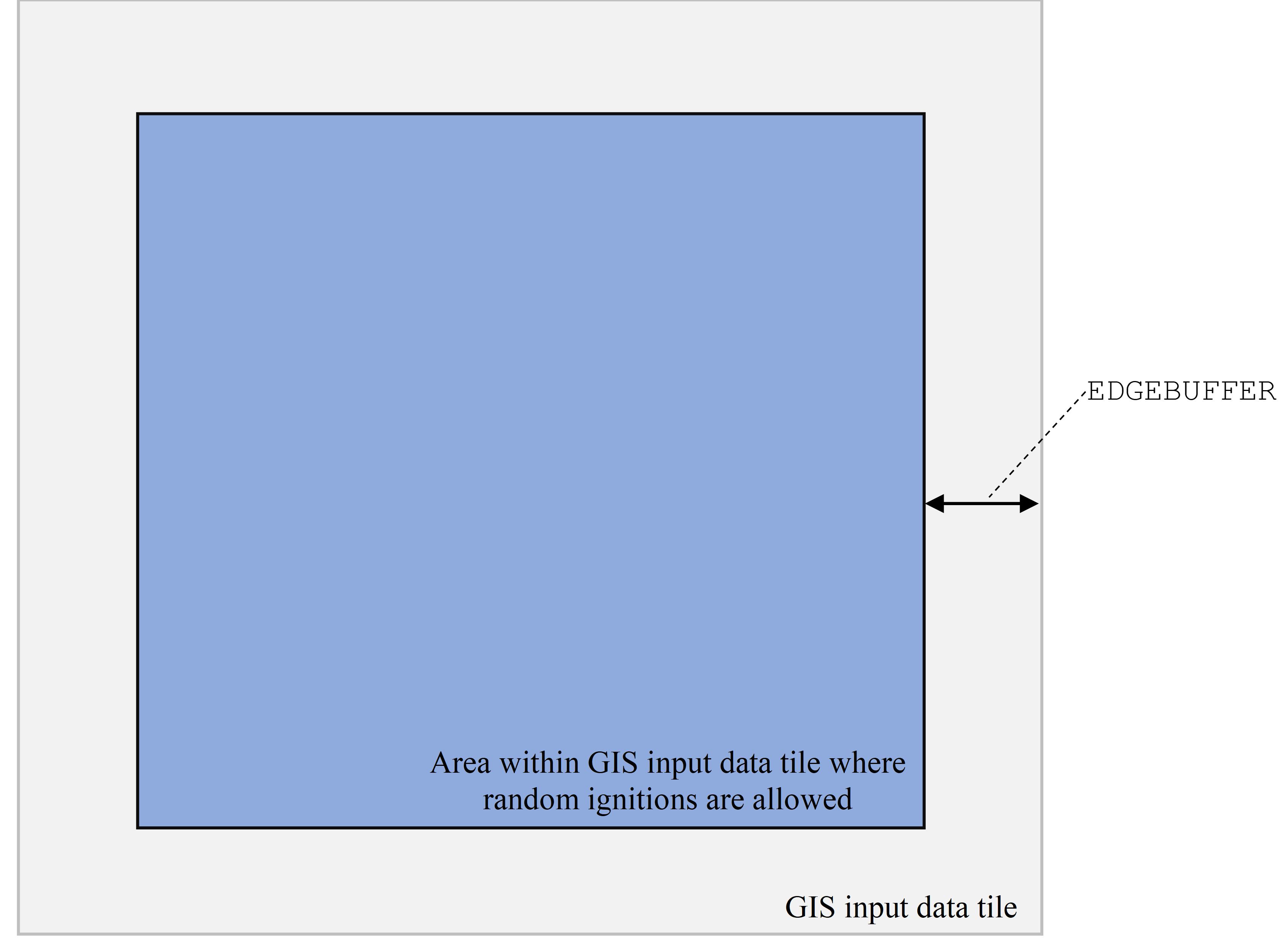
Setting RANDOM_IGNITIONS = .TRUE. directs ELMFIRE to conduct a Monte
Carlo analysis with ignition locations distributed randomly within the
computational domain. Allowable locations of those ignitions are
constrained by the parameter EDGEBUFFER which is the distance from
the edge of the GIS input data tile where ignitions will not be placed
as shown graphically below:
Random ignition location may also be constrained by an ignition mask
raster. To do this, set USE_IGNITION_MASK = .TRUE. and specify
IGNITION_MASK_FILENAME on the &INPUTS line. This directs ELMFIRE
to read a Float32 raster named IGNITION_MASK_FILENAME.tif from the
FUELS_AND_TOPOGRAPHY_DIRECTORY. Distribution of ignitions across the
landscape is controlled by the parameter RANDOM_IGNITIONS_TYPE:
RANDOM_IGNITIONS_TYPE=1(default): Ignitions are spatially distributed uniformly across the landscape in any pixels where the ignition mask raster is greater than zero. This is useful for modeling ignitions originating from powerlines or roads, for example.
RANDOM_IGNITIONS_TYPE=2: Ignitions are spatially distributed across the landscape at a density that is proportional to the ignition mask raster. This is useful for burn probability modeling where some locations across the landscape have higher ignition probabilities than other locations.
The number of randomly-generated ignition points can be specified in two ways:
By directly specifying
NUM_ENSEMBLE_MEMBERS, orBy specifying
PERCENT_OF_PIXELS_TO_IGNITEand settingNUM_ENSEMBLE_MEMBERSto a value less than 0.
In the first case, ELMFIRE will randomly generate
NUM_ENSEMBLE_MEMBERS ignition locations in the allowable ignition
area as defined by EDGEBUFFER (and, if USE_IGNITION_MASK =
.TRUE., the user-specified ignition mask raster as well). In the
second case, ELMFIRE will count all pixels within the allowable ignition
area and randomly ignite the user-specified percent of those pixels. In
some cases, a pixel may be selected more than once to be ignited. This
can be disabled by setting ALLOW_MULTIPLE_IGNITIONS_AT_A_PIXEL =
.FALSE..
Randomized weather streams
In the example discussed in Randomized ignition locations, ignition locations are selected randomly and a single weather stream (hindcast or forecast) is provided as input to those simulations. Often, as part of a climatological fire risk analysis, it is desirable to simulate wind and weather conditions under a range of historical (or forecasted) wind and weather conditions. This can be accomplished in ELMFIRE using stacked/multiband weather/meteorology rasters.
The manner in which these rasters are used is controlled by the
parameters NUM_METEOROLOGY_TIMES, METEOROLOGY_BAND_START,
METEOROLOGY_BAND_STOP, and METEOROLOGY_BAND_SKIP_INTERVAL. This
is perhaps best illustrated by an example. Assume that numerical weather
prediction has been used to generate 100 24-hour “blocks” of historical
wind/weather data at hourly intervals that will be provided as input to
a Monte Carlo analysis. The goal is to simulate 24-hours of fire spread,
for each of these 24-hour blocks. However, these 24-hour blocks are not
temporally contiguous, meaning the first 24-hour block could be from
August 1983 and the next 24-hour block could be from October 2012, and
so on.
Each 24-hour block consists of 25 bands since Band 1 is \({t}\) = 0
and Band 25 is \({t}\) = 24 hours. Therefore, each meteorology
raster would contain 2,500 separate bands (100 blocks \(\times\) 25
bands per block). Since ELMFIRE needs 25 bands of wind/weather data to
drive each 24-hour simulation, we would set METEOROLOGY_BAND_START=1,
METEOROLOGY_BAND_STOP=2476, and
METEOROLOGY_BAND_SKIP_INTERVAL=25. This tells ELMFIRE to use every
25th band as the starting band for a 24-hour simulation and ensures that
each 24-hour simulation starts with Band 1, 26, 51, and so on until the
final 24-hour block is reached at meteorology band 2476.
If, instead, the 100 24-hour blocks were temporally contiguous (for
example, a continuous hindcast from mid-July through the end of October)
and the purpose of the Monte Carlo analysis is to ignite fires every 3
hours and model their spread, we would set
METEOROLOGY_BAND_SKIP_INTERVAL=4.
Spatial and temporal perturbations of input rasters
All inputs are subject to inherent uncertainty. To address this uncertainty, input rasters may be perturbed stochastically from their baseline values in a Monte Carlo analysis. Currently, the following rasters may be perturbed:
ADJ: Spread rate adjustment factor (-)
CBD: Canopy bulk density (kg/\({m^3}\))
CBH: Canopy base height (m)
CC: Canopy cover (-)
CH: Canopy height (m)
FMC: Foliar moisture content (-)
M1: 1-hour fuel moisture (-)
M10: 10-hour fuel moisture (-)
M100: 100-hour fuel moisture (-)
MLH: Live herbaceous fuel moisture (-)
MLW: Live woody fuel moisture (-)
WAF: Wind adjustment factor (-)
WD: Wind direction (deg)
WS: Wind speed (mph)
Parameters controlling stochastic perturbations of input rasters are
specified in the &MONTE_CARLO namelist group. A random sampling
procedure is implemented such that the spatial perturbation to be
applied to a given input raster sampled from a probability density
function (pdf). Currently, only a uniform pdf is implemented
(PDF_TYPE(:) = 'UNIFORM') although this will eventually be
generalized to additional distributions such as Gaussian and lognormal.
The keyword NUM_RASTERS_TO_PERTURB prescribes the number of input
rasters to be perturbed and the keyword RASTER_TO_PERTURB(:) is a
string corresponding to one of the raster names in the bulleted list
above (ADJ, CBD, etc.). As an example, consider the following
lines:
NUM_RASTERS_TO_PERTURB   = 1
RASTER_TO_PERTUB(1)      = 'ADJ'
SPATIAL_PERTURBATION(1)  = 'GLOBAL'
TEMPORAL_PERTURBATION(1) = 'STATIC'
PDF_TYPE(1)              = 'UNIFORM'
PDF_LOWER_LIMIT(1)       = -0.10
PDF_UPPER_LIMIT(1)       = 0.10
These lines specify that a randomly selected value between -0.1 and 0.1
should be added to the spread rate adjustment factor(ADJ). This
perturbation will be applied globally to all pixels
(SPATIAL_PERTURBATION = 'GLOBAL') and is temporally invariant for
the duration of the simulation (TEMPORAL_PERTURBATION = 'STATIC').
Rather than applying such perturbations globally to all pixels,
different perturbations can be applied to different pixels by setting
SPATIAL_PERTURBATION = 'PIXEL'. Some raster inputs, such as wind
speed and direction, are multi-band rasters that vary temporally.
Different perturbations may be applied at each time by setting
TEMPORAL_PERTURBATION = 'DYNAMIC'. Normally, this would only be done
for wind speed and direction.
The number of ensemble members in the Monte Carlo analysis should be
specified using the keyword NUM_ENSEMBLE_MEMBERS (&MONTE_CARLO
namelist group). However, when using randomly-placed ignitions it may
instead be preferable to specify the total number of ensemble members by
specifying the percentage of pixels within the computational domain and
possibly within a user-specified ignition mask to ignite. This is
described in Randomized ignition locations.
Randomized wind fluctuation intensities
Wind fluctuations are implemented via the &SIMULATOR namelist group.
The keywords that control these fluctuations are
WIND_SPEED_FLUCTUATION_INTENSITY and
WIND_DIRECTION_FLUCTUATION_INTENSITY. These values can be randomized
by setting the following four parameters (in the &MONTE_CARLO
namelist group):
WIND_DIRECTION_FLUCTUATION_INTENSITY_MIN: Minimum wind direction fluctuation intensity value
WIND_DIRECTION_FLUCTUATION_INTENSITY_MAX: Maximum wind direction fluctuation intensity value
WIND_SPEED_FLUCTUATION_INTENSITY_MIN: Minimum wind speed fluctuation intensity value
WIND_SPEED_FLUCTUATION_INTENSITY_MAX: Maximum wind speed fluctuation intensity value
The wind fluctuation intensities are then randomly generated according to a uniform probability density function, with the upper and lower values specified by the above four parameters.
Outputs
Several outputs are specific to Monte Carlo analyses. Often, when
conducting a Monte Carlo analysis with randomly distributed ignitions,
it is informative to view spatial burn probabilities, defined as the
fraction of simulations in which a given pixel burned. To enable this
calculation (which adds some computational and network overhead), set
CALCULATE_BURN_PROBABILITY = .TRUE. in the &OUTPUTS namelist
group. This instructs ELMFIRE to aggregate all simulated fire perimeters
and calculate the burn probability across all runs and write the results
to disk (in a file called burn_probability.tif). The output raster
has three bands. The first is the conventional burn probability. The
second is passive crown fire burn probability, meaning the fraction of
times in which a pixel burned as passive crown fire. The third band is
active crown fire burn probability.